


Version [93341]
Dies ist eine alte Version von TutoriumGrundlagenStatistikHistogramm erstellt von FabianEndres am 2019-01-29 19:19:50.
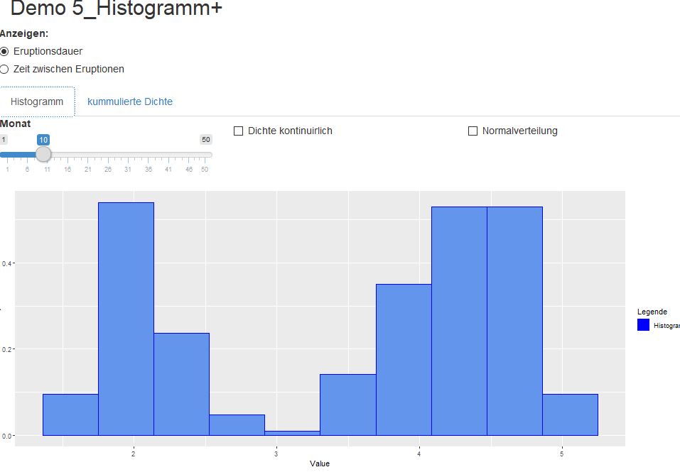
Histogramm
Für die Aufgabe Histogramm benötigen sie die Bibliothek staTools, laden sie diese bitte vor Beginn herunter.
server.R
library(shiny)
library(ggplot2)
library(staTools)
server <- function(input, output) {
data <- faithful
output$showAttribute <- renderUI({
radioButtons(inputId = 'showAttribute', label = 'Anzeigen: ',
choiceNames = c('Eruptionsdauer', 'Zeit zwischen Eruptionen'),
choiceValues = c(1, 2)
)
})# Tab 1 Histogramm
output$bins <- renderUI({
sliderInput(inputId = 'bins', label = 'Monat',
min = 1, max = 50, step = 1,
value = 10
)
})output$showDensity <- renderUI({
checkboxInput(inputId = "showDensity", label = "Dichte kontinuirlich", value = FALSE)
})output$showNorm <- renderUI({
checkboxInput(inputId = "showNorm", label = "Normalverteilung", value = FALSE)
})output$histogram <- renderPlot({
p <- ggplot(data.frame(Value = data[, as.numeric(input$showAttribute)]), aes(x = Value)) +
geom_histogram(aes(y = ..density.., colour = "Histogram"),
fill = "cornflowerblue",
bins = input$bins)
colourScaleValues = c("Histogram" = 'blue')
if (input$showDensity == TRUE) {
p <- p + geom_density(aes(colour = "Dichte"))
colourScaleValues <- c("Dichte" = 'black', colourScaleValues)
}
if (input$showNorm == TRUE) {
p <- p + stat_function(fun = dnorm, args = list(
mean = mean(data[, as.numeric(input$showAttribute)]),
sd = sd(data[, as.numeric(input$showAttribute)])
),
aes(colour = "Normalverteilung")
)
colourScaleValues <- c(colourScaleValues, "Normalverteilung" = 'red')
}
p <- p + scale_colour_manual(name = "Legende", values = colourScaleValues) +
guides(colour = guide_legend(override.aes = list(fill = colourScaleValues)))
p
})# Tab 2
output$showNorm_tab2 <- renderUI({
checkboxInput(inputId = "showNorm_tab2", label = "Normalverteilung", value = FALSE)
})output$densityPlot <- renderPlot({
data_cdf <- as.data.frame(cdf(data[, as.numeric(input$showAttribute)]))
normalDistribution <- data.frame(x = data[, as.numeric(input$showAttribute)],
y = pnorm(data[, as.numeric(input$showAttribute)],
mean = mean(data[, as.numeric(input$showAttribute)]),
sd = sd(data[, as.numeric(input$showAttribute)])))
p <- ggplot(data = data_cdf, aes(x = x, y = y)) +
geom_point(aes(colour = 'kummulierte Dichte')) +
scale_x_continuous(name = "Messwert") + # Label der x-Achse
scale_y_continuous(name = "kumulierte Wahrscheinlichkeit") # Label der y-Achse
if (input$showNorm_tab2 == TRUE) {
p <- p + geom_line(data = normalDistribution, aes(x = x, y = y, colour = 'Normalverteilung')) +
scale_colour_manual(name = "Legende", values = c('kummulierte Dichte' = 'black', 'Normalverteilung' = 'red'))
}
else {
p <- p + scale_colour_manual(name = "Legende", values = c('kummulierte Dichte' = 'black'))
}
p
})}
ui.R
ui <- fluidPage(
titlePanel("Demo 5_Histogramm+"),
fluidRow(htmlOutput('showAttribute')),
fluidRow(
tabsetPanel(
tabPanel('Histogramm',
fluidRow(
column(4, htmlOutput('bins')),
column(4, htmlOutput('showDensity')),
column(4, htmlOutput('showNorm'))
),
fluidRow(
plotOutput('histogram')
)
),
tabPanel('kummulierte Dichte',
fluidRow(
column(4, htmlOutput('showNorm_tab2'))
),
fluidRow(
plotOutput('densityPlot')
)
)
)
))
app.R
source('server.R', encoding = "UTF-8")
source('ui.R', encoding = "UTF-8")
shinyApp(ui = ui, server = server)
Hier können Sie den Quellcode ohne Kommentare zusammengefasst herunterladen:
Histogramm als .txt
| File | Last modified | Size |
|---|---|---|
| Histogramm.jpg | 2023-10-06 18:37 | 51Kb |
| Histogramm.txt | 2023-10-06 18:37 | 4Kb |
| << Zurück | >> Zur Übersicht |
<< Zurück zur Übersicht: Tutorium Grundlagen Statistik
CategoryTutorienFKITWS1819
Diese Seite wurde noch nicht kommentiert.